Kartikeya Sharma, Meryem Abouali, Tarek Saadawi

City University of New York, City College, New York, NY, 10031

[email protected], [email protected], [email protected]

Abstract

Around 1 in 10 Americans have diabetes according to the CDC while 90-95% of them have type-2 diabetes. Type-2 diabetes can be managed with regular in-person appointments. However, there are many situations in which in-person appointments are not possible due to affordability, accessibility to healthcare across the country, or a shortage of qualified healthcare professionals. This research project focuses on how machine learning can be utilized to better predict type-2 diabetes. The objective is to train a large dataset alongside various machine learning models and use the most performant one to help predict if an individual has type-2 diabetes or not. By the end of the research project, given a dataset with features such as age, weight, BMI, race, etc. the trained model will be able to predict, with a level of certainty, the probability of a patient having diabetes. After conducting the training, our findings revealed that the most performant machine learning technique was gradient boosting, giving a classification accuracy of 85%. To increase the accuracy further, future work includes simplifying the dataset, testing the trained model against different datasets, adding/removing some features, and connecting our model to a GUI to collect more data.

Background/Motivation

According to the CDC, about 1 in 10 Americans have diabetes, while 90-95% of them have type-2 diabetes^[1]. However, unlike many other diseases, diabetes can mostly be self-managed with additional support from your doctor. The problem arises when regular in-person appointments are not possible due to affordability, accessibility to healthcare across the country, or a shortage of qualified healthcare professionals. For example, during Summer 2020, medical professionals said they struggled to keep patients’ diabetes under control when regular in-person appointments were canceled or limited because of the COVID-19 pandemic. According to a new government study, nearly 40% of people who have died with COVID-19 had diabetes. Such circumstances require a call-to-action to provide greater innovation in the field of healthcare. One innovative solution is to use machine learning to help identify patients who have type-2 diabetes. In places or situations, where in-person appointments are not possible, machine learning can be used to inform patients about any potential risks they may face early on.

Current research on predicting type-2 diabetes using machine learning includes training on datasets that are outdated, small, or from outside the United States. This research project aims to provide a reliable machine learning model to predict type-2 diabetes while being trained on relevant and credible sources within the United States.

Methodology

The Dataset

In order to train a machine learning model to accurately predict type-2 diabetes, we must first find a large dataset. Since we are training on sensitive information and our target audience is individuals in the United States, the data must be relevant and be from a credible source. For this project, we have chosen a dataset from The National Health and Nutrition Examination Survey (NHANES) which is a program of studies designed to assess the health and nutritional status of adults and children in the United States. The study was carried out by the National Center for Health Statistics (NCHS) which is part of the Centers for Disease Control and Prevention (CDC).

To ensure we can train on a large enough dataset, we have chosen data from the latest three consecutive years: 2013-2014 (5,061 entries), 2015-2016 (4,860 entries), 2017-2018 (729 entries). After researching various sources^{[2] [3] [4]} and by looking at the features provided by NHANES, we decided to include these features for training:

• Total cholesterol (mg/dL) [NHANES code: LBXTC]
• Age [NHANES code: RIDAGEYR]
• Waist Circumference (cm) [NHANES code: BMXWAIST]
• Family history – If any of your blood relatives were told by a health professional that they have diabetes [NHANES code: MCQ300c]
• Race [NHANES code: RIDRETH3]
• Standing Height (cm) [NHANES code: BMXHT]
• Weight (kg) [NHANES code: BMXWT]
• Body Mass Index (kg/m**2) [NHANES code: BMXBMI]
• Hypertension – If you have ever been told by a health professional that you had high blood pressure [NHANES code: BPQ020]
• Physical activity – Do you do any moderate-intensity sports, fitness, or recreational activities for at least 10 minutes continuously daily [NHANES code: PAQ665]

Once all the data is imported locally, the dataset must then be cleaned. We need to remove any null, zero, empty, and irrelevant values. We will then split our dataset in a 75% train set and a 25% test set. The training set will be used to train the various machine learning algorithms while the testing set will be used to calculate the performance metrics and the overall classification accuracy.

Machine Learning Algorithms

We plan on using various machine learning models to train our testing set. This will allow us to compare the performance metrics of the most performant ones and tune it further. Since we are working with a supervised learning model (binary classification), the machine learning algorithms we will train are:

• KNeighborsClassifier
• LogisticRegression
• SVC
• LinearSVC
• RandomForestClassifier
• DecisionTreeClassifier
• GradientBoostingClassifier
• MLPClassifier
• GaussianNB

Performance Metrics

Before we choose the most accurate model, we must decide on performance metrics that should be used to rank the accuracy of each. The performance metrics we have chosen are:

• Classification Accuracy
• Precision
• Recall
• F1 Score

Analysis & Discussion

The Dataset

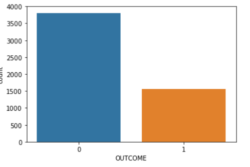
After extracting, processing, and classifying the data, we ended up with data on 5,368 individuals. From those, 3,808 individuals had an outcome value of 0 (don’t have diabetes) and 1,560 individuals had an outcome value of 1 (have diabetes):

Next, we split the data into a 75% training set and 25% testing set:

// create training and testing variables

X_train, X_test, y_train, y_test = train_test_split(diabetes.loc[:, diabetes.columns != 'OUTCOME'], diabetes['OUTCOME'], stratify=diabetes['OUTCOME'], random_state=42)

Training on dataset

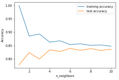
After splitting the dataset, we need to train different models on the dataset and understand how each algorithm works on a basic level. For example, to calculate the classification accuracy of the KNeighborsClassifier model, we need to first figure out how many neighbors are needed to give the highest training and testing accuracy. Below is a graph displaying how the training and testing accuracy differ as the number of neighbors to use by default for kneighbors queries changes:

A similar approach was used for other models and the final classification accuracy results are presented below:

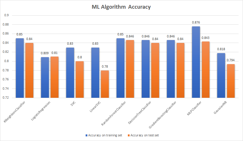
With a cutoff of around 84%, some models were studied at a deeper level by calculating their performance metrics to understand which model might be ideal to tune further. The top 5 models are listed below with their performance metric scores:

Model	Precision	Recall	F1-Score	Classification Accuracy
KNeighborsClassifier	0.860	0.840	0.820	0.840
RandomForestClassifier	0.870	0.850	0.830	0.846
DecisionTreeClassifier	0.870	0.840	0.820	0.840
GradientBoostingClassifier	0.850	0.850	0.840	0.840
MLPClassifier	0.810	0.810	0.810	0.843

By looking at our performance metrics, the GradientBoostingClassifier model had the most consistent accuracy when compared with the other four. The next step was to tune additional parameters of the gradient boosting technique to improve the overall classification accuracy. We will be tuning:

1. The learning rate – Shrinks the contribution of each tree by the learning rate
2. The max depth – Maximum depth of the individual regression estimators
3. The n estimators value – The number of boosting stages to perform

To find the best learning_rate value, we will simply train our GradientBoostingClassifier model with different learning rates and see which one had the highest validation accuracy score. We also want to make sure that the training accuracy score is as close as possible to the validation accuracy score to prevent overfitting/underfitting. From our results (Appendix 1), we noticed that the validation accuracy score was highest when the learning_rate was 0.15. From here, we can find out what max_depth value provides the highest validation accuracy score given a learning_rate of 0.15. From our results (Appendix 2), we saw that a max_depth value of 4 gave the highest validation accuracy score. We can use our previous findings: learning_rate=0.15 and max_depth=4 to finally see which n_estimators value gives the highest validation accuracy score. The best n_estimators value was recorded to be 100 (Appendix 3).

As a result, the validation accuracy score was highest when the learning_rate was 0.15, the max_depth was 4, and the n_estimators was 100. We can use these parameter values to calculate a tuned classification accuracy of our GradientBoostingClassifier model.

Conclusion

From our results, we saw that the validation accuracy was highest when the learning_rate was 0.15, the max_depth was 4, and the n_estimators was 100. From these parameter values, we can re-train our X_train variable and use the testing set to predict the classification accuracy.

Our final accuracy was 85% (Appendix 4). To conclude, given a dataset with features such as age, weight, BMI, race, etc. our trained model can predict, with an 85% level of certainty, the probability of a patient having type-2 diabetes.

Future Work

After working on this research project, there are many learnings that we can use to improve the accuracy of the type-2 diabetes prediction algorithm above 85%. They include:

• Simplifying the dataset – When we tried to tune the gradient boosting technique further, we noticed that the classification accuracy did not improve drastically. One reason for a lack of improvement is because the decision tree that is used to make the prediction is too crowded (Appendix 5). To improve accuracy, we need to improve the overall feature importance score by utilizing different calculation methods.

• Test model against different datasets – To make sure our machine learning model is not overfitted, we should test it against other datasets. Achieving a high accuracy across various datasets will allow our model to generalize to unseen data outside the training set.

• Test with different features – For best results, we should add/remove features from our dataset and see how the model performs based on these changes. This will also provide insight on which features influence the prediction most.

• Connect model to a GUI – To regularly collect more data and make our model available to the public, future work includes connecting our model with a front-end GUI for better user experience.

Acknowledgment

This research was supported by the Opportunities in Research and Creative Arts Program (ORCA). I would also like to thank my mentor Tarek Saadawi and Meryem Abouali for their guidance and supervision on the completion of this project.

References

Code repository: https://github.com/kartikeya01/diabetes-ml

Appendix

Appendix 1

learning_rate_list = [0.15, 0.1, 0.05, 0.01, 0.005, 0.001]

for learning_rate in learning_rate_list:
    gb_clf = GradientBoostingClassifier(n_estimators=20, learning_rate=learning_rate, max_features=2, max_depth=2, random_state=0)
    gb_clf.fit(X_train, y_train)

    print("Learning rate: ", learning_rate)
    print("Accuracy score (training): {0:.3f}".format(gb_clf.score(X_train, y_train)))
    print("Accuracy score (validation): {0:.3f}".format(gb_clf.score(X_test, y_test)))

// RETURN:

[BEST] ('Learning rate: ', 0.15)
Accuracy score (training): 0.855
Accuracy score (validation): 0.848

('Learning rate: ', 0.1)
Accuracy score (training): 0.846
Accuracy score (validation): 0.842

('Learning rate: ', 0.05)
Accuracy score (training): 0.814
Accuracy score (validation): 0.812

('Learning rate: ', 0.01)
Accuracy score (training): 0.709
Accuracy score (validation): 0.709

('Learning rate: ', 0.005)
Accuracy score (training): 0.709
Accuracy score (validation): 0.709

('Learning rate: ', 0.001)
Accuracy score (training): 0.709
Accuracy score (validation): 0.709

Appendix 2

max_depth_list = [2, 3, 4, 5, 6, 7]

for max_depth in max_depth_list:
    gb_clf = GradientBoostingClassifier(n_estimators=20, learning_rate=0.15, max_features=2, max_depth=max_depth, random_state=0)
    gb_clf.fit(X_train, y_train)

    print("Max depth: ", max_depth)
    print("Accuracy score (training): {0:.3f}".format(gb_clf.score(X_train, y_train)))
    print("Accuracy score (validation): {0:.3f}".format(gb_clf.score(X_test, y_test)))

// RETURN:

('Max depth: ', 2)
Accuracy score (training): 0.855
Accuracy score (validation): 0.848

('Max depth: ', 3)
Accuracy score (training): 0.858
Accuracy score (validation): 0.852

[BEST] ('Max depth: ', 4)
Accuracy score (training): 0.867
Accuracy score (validation): 0.854

('Max depth: ', 5)
Accuracy score (training): 0.880
Accuracy score (validation): 0.852

('Max depth: ', 6)
Accuracy score (training): 0.893
Accuracy score (validation): 0.852

('Max depth: ', 7)
Accuracy score (training): 0.922
Accuracy score (validation): 0.853

Appendix 3

n_estimators_list = [100, 250, 500, 750, 1000, 1250, 1500, 1750]

for n_estimators in n_estimators_list:
    gb_clf = GradientBoostingClassifier(n_estimators=n_estimators, learning_rate=0.15, max_features=2, max_depth=4, random_state=0)
    gb_clf.fit(X_train, y_train)

    print("N estimators: ", n_estimators)
    print("Accuracy score (training): {0:.3f}".format(gb_clf.score(X_train, y_train)))
    print("Accuracy score (validation): {0:.3f}".format(gb_clf.score(X_test, y_test)))

// RETURN:

[BEST] ('N estimators: ', 100)
Accuracy score (training): 0.913
Accuracy score (validation): 0.844

('N estimators: ', 250)
Accuracy score (training): 0.962
Accuracy score (validation): 0.842

('N estimators: ', 500)
Accuracy score (training): 0.997
Accuracy score (validation): 0.840

('N estimators: ', 750)
Accuracy score (training): 1.000
Accuracy score (validation): 0.836

('N estimators: ', 1000)
Accuracy score (training): 1.000
Accuracy score (validation): 0.838

('N estimators: ', 1250)
Accuracy score (training): 1.000
Accuracy score (validation): 0.836

('N estimators: ', 1500)
Accuracy score (training): 1.000
Accuracy score (validation): 0.833

('N estimators: ', 1750)
Accuracy score (training): 1.000
Accuracy score (validation): 0.837

Appendix 4

from xgboost import XGBClassifier

xgb_clf = XGBClassifier(learning_rate=0.15, max_depth=4, n_estimators=100)
xgb_clf.fit(X_train, y_train)

score = xgb_clf.score(X_test, y_test)
print(score)

// RETURN:

0.8502235469448585

Appendix 5